Warning: this post is terribly technical. Readers not inclined towards statistical analysis and R coding may wish to skip this one!

I was recently contacted by a biologist in the UK regarding one of the analyses that I did in my PhD. This researcher was trying to model percentage data with mixed effects models and was struggling to find examples of where this had been done before to base his analysis on, except for the analysis that I performed to identify drivers of disturbance at a patch level in the Great Western Woodlands. I remember that at the time, I really struggled to figure out the best way to perform the analysis, it was so complicated and there were issues that made it different from all the other examples I was trying to go off. I remember assuming that it was probably really straightforward and that everyone else does these sorts of analyses all the time and that I was a bit slow for not being able to figure it out straight away… so it is somewhat gratifying to hear that it’s not a common problem that biologists solve, and to have someone else reaching out to me for my experience on it!

I’ve decided to write up my response as a blog post, in case anyone else is interested… and to remind myself of what happened there! Comments and suggestions for improvement are invited!

In general terms, the analysis is aimed at understanding what factors explain how much anthropogenic disturbance (e.g. land clearing) will occur within the landscapes of the Great Western Woodlands, where there is an abundance of mining activity and pastoralism within an otherwise relatively undisturbed region.

More specifically, the analysis relates to predicting the percentage of area disturbed (the ‘development footprint’) at a patch level (this was the smaller of two scales of analysis used in the investigation, and the only one to be discussed here), by a set of potential predictor variables. The predictor variables included both categorical and continuous variables. Categorical variables were: pastoral tenure, greenstone lithology, conservation estate, ironstone formation, schedule 1 area clearing restrictions, environmentally sensitive area designation, vegetation formation, type of tenements (exploration/prospecting tenement, mining and related activities tenement, none), primary target commodity (gold, nickel, iron-ore, other), and sample area (n=24). The numerical variables were: number of mining projects, number of dead tenements, sum of duration of all live and dead tenements, distance to wheatbelt, and distance to nearest town.

The next image (below) shows an example of these patches and their attribuets.

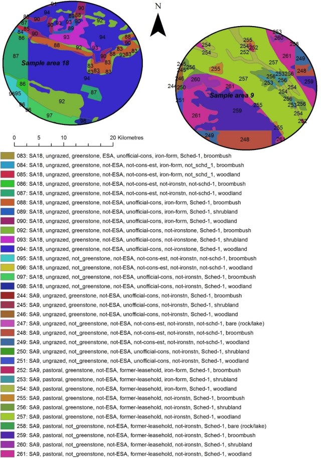
Example of polygons constructed to assess predictors of development footprint at the patch level

I used ‘nlme’ package in R for the analysis. Early in the data exploration (which I won’t detail here) I realised that the data for the proportional area disturbed was very skewed, and that log or other transformations weren’t enough to achieve a normal-ish distribution. A logistic transformation was the clear solution, given the percentage nature of the data (i.e. that it was bounded by 0 and 1); see the following image with scatter plots and histograms.

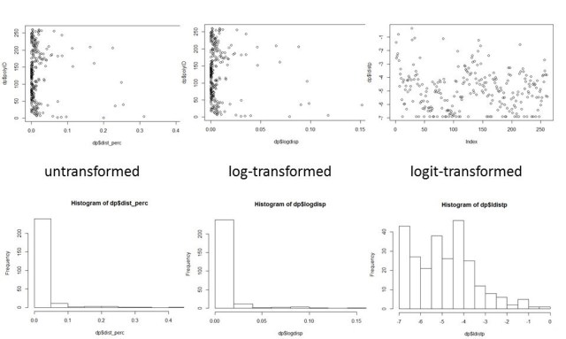
However, I couldn’t just use a GLMM with a gaussian distribution and a logit link, as this would have produced the problem that predicated values will be outside the 0-1 range. I had to first do a logistic transformation, model linearly, and then back-transform the modelled values.

The following line of code shows how I logit-transformed the proportion of area disturbed (‘dist_perc’), after adding 0.001 to each value (I had to do this as logit only works on values between 0 and 1, exclusive). I also show how I ‘untranformed’ the data and plotted it to produce a nice, normal, histogram. Note that dp was the dataframe I worked with, stands for ‘disturbance by patch’.

> dp$ldistp = qlogis(dist_perc+0.001)                   # qlogis does a logit transformation on (a set of) values.

> plot(dp$ldistp)                                         # scatter plot looks much better

> range(dp$ldistp)

> hist(dp$ldistp)                                         # Looks good.

> dp$s.dist = scale(dp$ldistp)                   # s.dist is the logit-transformed, scaled disturbed percentage

> back_transformed = (plogis(dp$ldistp))-0.001           # plogis ‘undoes’ the logit transformation.

After completion of the data exploration and dealing with other variables that needed to be transformed, confirming no outliers, dealing with collinearity etc and scaling issues, I modelled the transformed variable using maximum likelihood and performed a manual backward-selection and a few other checks to reach the final model, which I then modelled using REML.

I have included the whole script here. It includes the data exploration stages, as well as a plethora of comments, and also a few tries of alternative analysis techniques using lmer, lmerTest and lme4 (and modelling with a logit-link before I figured out that this wasn’t a useful approach). I take no responsibility for errors! Check line 621 for the final model, followed by back-transformations of the outcomes.