Sustaining Ecology

Note: this is a post to hold the R script that is referred to in this post. It’s even more awfully technical than the post that refers to it; readers not interested or familiar with R code or this type of analysis may want to skip it!

You’d probably want to copy this all in to an R script (and perhaps view in r studio) to make sense of it.

# Disturbance by patch to determine landscape predictors of disturbance —-

# Housekeeping —-
setwd(“C:/Users/ke/Dropbox/PhD/Chapter 3 – spatial analysis/R”)
library(lme4); library(ggplot2); library(plyr); library(lattice); library(car); require(lmerTest); library(nlme)
source(“HighstatLibV6.R”)
dp

# Start of data exploration —-
names(dp)
str(dp)
summary(dp)
attach(dp)
head(dp)
sum(is.na(dp)) # no missing values

# 4.2 looking for outliers
vars1 “greenstone” , “esa” , “cons_estate” , “iron_formation”)
Mydotplot(dp[, vars1])
vars2 “mining_activity”,”commodity”,”wheatbelt_dist”,”town_dist”,”patch_area”,”disturbed.area”, “dist_perc”)
Mydotplot(dp[, vars2])
vars3 Mydotplot(dp[, vars3])
# no outliers once the tenement years issue was fixed (in raw data), but some vars need transformation

# Transforming variables —-

# mini-tutorial on how scaling works:
x s.x s.x # the resultant scaled variable stored the scaling attributes: the centre (mean) and scale (multiplier)
attr(s.x,”scaled:center”) # 5.5; extracting the centre, the mean of the original vector, from which each value was subtracted to do the scaling
attr(s.x,”scaled:scale”) # 3.02765; extracting the scale (the multiplier)
x.recreated = s.x*attr(s.x,’scaled:scale’) + attr(s.x,’scaled:center’) # to unscale just multiply the scaled vector by the ‘scale’ and add the ‘centre’

# transforming disturbance percentage:
plot(dp$polyID~dp$dist_perc)
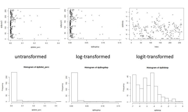
hist(dp$dist_perc) # too skewed
dist_perc1 = dist_perc + 1
dp$logdisp = log(dist_perc1)
range(dp$logdisp)
hist(dp$logdisp)
plot(dp$polyID~dp$logdisp) # still too squashed. try log10 transformation?
dp$logdisp = log10(dist_perc1)
attach(dp)
range(dp$logdisp)
hist(dp$logdisp)
plot(dp$polyID~dp$logdisp) # still too skewed. Let’s try a logit transformation:
qlogis(0.9) # Getting familiar w logit transformations… this returns 2.197. qlogis does a logit transformation on (a set of) values.
plogis(2.197225) # returns 0.9. plogis ‘undoes’ the logit transformation.
dp$ldistp = (qlogis(dp$dist_perc+0.001)) # ldistp is logit transformation of the percent disturbed plus 0.001
plot(dp$ldistp) # Looks good.
range(dp$ldistp)
hist(dp$ldistp)
dp$s.dist = scale(dp$ldistp) # s.dist is the logit-transformed, scaled disturbed percentage
hist(dp$s.dist)
# OK I need to either do a logistic regression here, or simply logit-transform the response before modelling linearly
# doing a logistic transformation and then modelling linearly – advised by Michael Renton

# transforming and scaling ten_yrs:
range(ten_yrs) # the 177 is a valid value.
plot(ten_yrs) # needs some transformation
dp$lntyrs = log((ten_yrs+1))
plot(dp$lntyrs) # yep the natural log looks good.
range(dp$lntyrs)
dp$s.lntyrs = scale(dp$lntyrs, center = TRUE, scale = TRUE)
plot(dp$lntyrs)
plot(dp$s.lntyrs)

# transforming patch area:
range(dp$patch_area)
dp$patchkm2 = dp$patch_area/1000000 # make kms instead of m2
range(dp$patchkm2)
hist(dp$patchkm2)
dp$ln.pkm = log(dp$patchkm2) # natural log of patch area
hist(dp$ln.pkm) # centred and normalish

# transforming minedex_count:
plot(minedex_count)
table(dp$minedex_count)
plot(log(minedex_count+1)) # somewhat better
logmx = log(minedex_count+1)
range(logmx)
dp$s.mx = scale(logmx)
plot(dp$s.mx)

# transforming distance to wheatbelt:
range(wheatbelt_dist)
dp$wbkm = wheatbelt_dist/1000
plot(dp$wbkm)
range(dp$wbkm)
dp$s.wb = scale(dp$wbkm)
plot(dp$s.wb)

# transforming distance to town:
dp$tnkm = town_dist/1000
plot(dp$tnkm)
range(dp$tnkm)
dp$s.tn = scale(dp$tnkm)
plot(dp$s.tn)

# not much can be done with the commodity variable:
summary(dp$commodity) # not sure if having the “no commodity stated” value is useful…
# dp$commodity[dp$commodity==”no commodity stated”] <- “none” # creates NAs

# adding second-order polynomials of the numerical variables
dp$tenyrs2 = dp$s.lntyrs^2
dp$mx2 = dp$s.mx^2
dp$wb2 = dp$s.wb^2
dp$tn2 = dp$s.tn^2
range(dp$s.lntyrs)
range(dp$tenyrs2)

# combining greenstone and ironstone lithology data into one categorical variable
dp$lithology = ifelse(greenstone == “greenstone”,”greenstone”,”other.lithology”)
dp$iron_formation
dp$lithology = ifelse(iron_formation == “iron-form”,”iron.formation”,dp$lithology)
dp$lithology
table(dp$lithology) # clever duck

# Looking for collinearity —-
pairs(dp[,vars1], lower.panel = panel.cor)
#i.e. SA number, SA_mines and category all related – use SA_mines
pairs(dp[,vars2], lower.panel = panel.cor)
miningvars = c(“SA_mines”,”greenstone”,”iron_formation”,”minedex_count”,”ten_yrs”,”mining_activity”,”commodity”)
pairs(dp[,miningvars], lower.panel = panel.cor)
# also strong collinearity between minedex count and dt-count, mined and
# note mining activity replaces expl_ten and mined.
# low 0.4 collinearity between minedex count and ten_yrs, and 0.5 between SA_mines and mining activity

summary(dp$dist_perc ~ dp$veg_form)
summary(dp$cons_estate)

dpvars = c(“pastoral”,”greenstone”,”esa”,”cons_estate”,”iron_formation”,”sched_1″,”veg_form”,
“mining_activity”,”commodity”,”s.mx”,”s.lntyrs”,”s.wb”,”s.tn”,”s.dist”)
Mydotplot(dp[, dpvars])
pairs(dp[,dpvars], lower.panel = panel.cor)
# ok, have dealt with collinearity. There’s nothing above 0.5, and even the 0.5 is not important

# looking at possible X Y relationships —-

# first the numeric variables: plot Y against the Xes and calculate pearson coefficients:
dpnumvars = c(“s.mx”,”s.lntyrs”,”s.wb”,”s.tn”,”s.dist”)
pairs(dp[,dpnumvars], lower.panel = panel.cor)
# there appears to be a positive relationship between the area disturbed and both the
# number of mining projects and the total duration of tenements in an area.
# No relation with distance from wheatbelt, and slight negative relationship with distance from town,
# which makes sense – areas near towns are more likely to get more disturbed and to stop tracks from growing over etc.

plot(dp$dist_perc~dp$lntyrs) #remember that dp$lntyrs = log((ten_yrs+1))
plot(dp$ldistp~dp$lntyrs)

#then categorical variables:
boxplot(dp$s.dist~dp$pastoral) # no real effect of pastoral activity
boxplot(dp$s.dist~dp$greenstone) # more disturbance on greenstone
boxplot(dp$s.dist~dp$esa) # more disturbance on ESAs
boxplot(dp$s.dist~dp$cons_estate) # greatest disturbance on former leasehold then class As!
# UCL has same mean distrubance as gazetted conservation estate; though higher variance.
boxplot(dp$s.dist~dp$iron_formation) # more disturbance on BIFs
boxplot(dp$s.dist~dp$sched_1) # more disturbance on schedule 1 areas
boxplot(dp$s.dist~dp$veg_form) # less disturbance in bare areas and succulent steppe
boxplot(dp$dist_perc~dp$veg_form)
boxplot(dp$s.dist~dp$mining_activity) # more disturbance where there’s been mining tenement.
# strangely similar between exploration and no mining tenement.
boxplot(dp$s.dist~dp$commodity) # most disturbance around gold mining projects, maybe not significant

# Looking for interactions —-

coplot(s.dist ~ s.mx | factor(commodity), data = dp)
# R displays from lower left, across, to upper right.

coplot(s.dist ~ s.mx | factor(commodity), data = dp,
panel = function(x, y, …) {
tmp abline(tmp)
points(x, y) })
# there could be an interaction between the commodity and the number of mining projects

coplot(s.dist ~ s.lntyrs | factor(pastoral), data = dp,
panel = function(x, y, …) {
tmp abline(tmp)
points(x, y) })
# There could be an interaction between tenement years and pastoral, same as found in regional-scale analysis.

coplot(s.dist ~ factor(greenstone) | factor(pastoral), data = dp,
panel = function(x, y, …) {
tmp abline(tmp)
points(x, y) })
# maybe nothing between greenstone and pastoral

coplot(s.dist ~ factor(veg_form) | factor(greenstone), data = dp,
panel = function(x, y, …) {
tmp abline(tmp)
points(x, y) })
# maybe nothing between greenstone and pastoral
coplot(s.dist ~ s.tn | factor(veg_form), data = dp,
panel = function(x, y, …) {
tmp abline(tmp)
points(x, y) })
# well there doesn’t seem to be much mallee near towns; looks like there could be an interaction

coplot(s.dist ~ s.tn | factor(esa), data = dp,
panel = function(x, y, …) {
tmp abline(tmp)
points(x, y) })
# definitely looks like an interaction between esas and dist to town

coplot(s.dist ~ s.wb | factor(esa), data = dp,
panel = function(x, y, …) {
tmp abline(tmp)
points(x, y) })
# same again – interaction between esas and distance to wheatbelt, although esas tend to be much closer to wheatbelt than non-esas.

coplot(s.dist ~ factor(veg_form) | factor(esa), data = dp,
panel = function(x, y, …) {
tmp abline(tmp)
points(x, y) })

coplot(s.dist ~ factor(mining_activity) | factor(veg_form), data = dp )
# most of the mining and exploration appears to be in woodland

# Fitting and selecting models —-

# 4.7.1 using gaussian family and logit link with lme4
# glmer example: model1 dp1 = glmer(dist_perc ~ factor(pastoral)+factor(greenstone)+factor(esa)+factor(cons_estate)+
factor(iron_formation)+factor(sched_1)+factor(veg_form)+factor(commodity)+
factor(mining_activity)+s.lntyrs+s.mx+s.wb+s.tn+
(1|SA_number),
data=dp, family = gaussian (link = ‘logit’))
summary(dp1)

E1 F1 plot(x = F1,
y = E1,
xlab = “Fitted values”,
ylab = “Residuals”,
main = “Homogeneity?”)
abline(h = 0, v = 0, lty = 2)
plot(dp1)
plot(F1)

# 4.7.2 Fitting a linear mixed model with a logit-transformed response in lmerTest
dp2 = lmer(s.dist ~ factor(pastoral)+factor(greenstone)+factor(esa)+factor(cons_estate)+
factor(iron_formation)+factor(sched_1)+factor(veg_form)+factor(commodity)+
factor(mining_activity)+s.lntyrs+s.mx+s.wb+s.tn+tenyrs2+mx2+wb2+tn2+
(1|SA_number), REML=TRUE,
data=dp)
summary(dp2)
plot(dp2)
summary(dp$commodity)
# dp$commodity[is.na(dp$commodity)] <- “none”

# compare with model that doesn’t have random effects to see if they are important
dp2.gls = gls(s.dist ~ factor(pastoral)+factor(greenstone)+factor(esa)+factor(cons_estate)+
factor(iron_formation)+factor(sched_1)+factor(veg_form)+factor(commodity)+
factor(mining_activity)+s.lntyrs+s.mx+s.wb+s.tn+tenyrs2+mx2+wb2+tn2,
data=dp)
summary(dp2.gls)
plot(dp2.gls)

anova(dp2.gls,dp2)
anova(dp2)

plot(dp2)
E2 F2 plot(x = F2,
y = E2,
xlab = “Fitted values”,
ylab = “Residuals”,
main = “Homogeneity?”)
abline(h = 0, v = 0, lty = 2)
table(dp$SA_number)
length(E2)

dp3 = lmer(s.dist ~ factor(pastoral)+factor(greenstone)+factor(esa)+factor(cons_estate)+
factor(iron_formation)+factor(sched_1)+factor(veg_form)+factor(commodity)+
factor(mining_activity)+s.lntyrs+s.mx+s.wb+s.tn+tenyrs2+mx2+wb2+tn2+
(1|SA_number),
data=dp, REML = FALSE)
summary(dp3)
anova(dp3)

dp4 = lmer(s.dist ~ factor(pastoral)+factor(greenstone)+factor(esa)+factor(cons_estate)+
factor(veg_form)+factor(commodity)+
factor(mining_activity)+s.lntyrs+s.mx+s.wb+s.tn+
(1|SA_number),
data=dp, REML = FALSE)
summary(dp4)
anova(dp4)

dp5 = lmer(s.dist ~ factor(pastoral)+factor(greenstone)+factor(esa)+factor(cons_estate)+
factor(veg_form)+
factor(mining_activity)+s.lntyrs+s.mx+s.wb+s.tn+
(1|SA_number),
data=dp, REML = FALSE)
summary(dp5)
anova(dp5)

dp6 = lmer(s.dist ~ factor(pastoral)+factor(greenstone)+factor(esa)+factor(cons_estate)+
factor(veg_form)+
factor(mining_activity)+s.lntyrs+s.mx+s.wb+s.tn+
(1|SA_number),
data=dp, REML = FALSE)
summary(dp6)
anova(dp6)

# 4.7.3 Fitting a linear mixed model with a logit-transformed response in nlme

library(nlme)
# first check the significance of the random effect structure:
dp1 = lme(s.dist ~ factor(pastoral)+factor(iron_formation)+factor(greenstone)+factor(esa)+factor(cons_estate)+
factor(sched_1)+factor(veg_form) +factor(commodity)+factor(mining_activity)+
s.lntyrs+s.mx+s.wb+s.tn+tenyrs2+mx2+wb2+tn2+ln.pkm,
random = ~1|SA_number,method = “REML”,
data=dp)
summary(dp1)
plot(dp1)

# compare with model that doesn’t have random effects to see if they are important
dp1.gls = gls(s.dist ~ factor(pastoral) +factor(iron_formation) +factor(greenstone) +factor(esa) +
factor(cons_estate) +factor(sched_1) +factor(veg_form) +factor(commodity) +
factor(mining_activity) +s.lntyrs +s.mx +s.wb +s.tn +tenyrs2 +mx2 +wb2 +tn2 +ln.pkm,
data=dp)
dp$s.dist
summary(dp1.gls)
plot(dp1.gls)

anova(dp1.gls,dpn1)
# The p-value of the Maximum Likelihood ratio test comparison between the mixed and fixed methods
# (both calculated using REML, which allows us to apply the likelihood ratio test) is 0.0154,
# indicating that the random factor is significant.

# check the model:
E2 F2 op MyYlab <- “Residuals”
plot(x = F2, y = E2, xlab = “Fitted values”, ylab = MyYlab, main=”Residuals versus fitted”)
boxplot(E2 ~ pastoral, data = dp,
main = “Pastoral tenure”, ylab = MyYlab)
boxplot(E2 ~ greenstone, data = dp,
main = “Greenstone lithology”, ylab = MyYlab)
plot(x = dp$s.lntyrs, y = E2, ylab = MyYlab,
main = “Tenement duration”, xlab = “scaled log of total tenement duration”)
par(op)
#haven’t checked against all variables but there’s too many, moving on for now and will check when model is smaller.

# Next, I’m going to fit the ‘beyond optimal’ model with ML, then reduce it manually
# then validate it,
dp2 = lme(s.dist ~ factor(pastoral)+factor(greenstone)+factor(esa)+factor(cons_estate)+
factor(iron_formation)+factor(sched_1)+factor(veg_form)+factor(commodity)+
factor(mining_activity)+s.lntyrs+s.mx+s.wb+s.tn+tenyrs2+mx2+wb2+tn2+ln.pkm,
random = ~1|SA_number,method = “ML”,
data=dp)
summary(dp2)

# remove tn2
dp3 = lme(s.dist ~ factor(pastoral)+factor(greenstone)+factor(esa)+factor(cons_estate)+
factor(iron_formation)+factor(sched_1)+factor(veg_form)+factor(commodity)+
factor(mining_activity)+s.lntyrs+s.mx+s.wb+s.tn+tenyrs2+mx2+wb2+ln.pkm,
random = ~1|SA_number,method = “ML”,
data=dp)
anova(dp2,dp3)

# remove mx2
dp4 = lme(s.dist ~ factor(pastoral)+factor(greenstone)+factor(esa)+factor(cons_estate)+
factor(iron_formation)+factor(sched_1)+factor(veg_form)+factor(commodity)+
factor(mining_activity)+s.lntyrs+s.mx+s.wb+s.tn+tenyrs2+wb2+ln.pkm,
random = ~1|SA_number,method = “ML”,
data=dp)
anova(dp4,dp3) #yes, wasn’t significant
summary(dp4)

# remove wb2
dp5 = lme(s.dist ~ factor(pastoral)+factor(greenstone)+factor(esa)+factor(cons_estate)+
factor(iron_formation)+factor(sched_1)+factor(veg_form)+factor(commodity)+
factor(mining_activity)+s.lntyrs+s.mx+s.wb+s.tn+tenyrs2+ln.pkm,
random = ~1|SA_number,method = “ML”,
data=dp)
summary(dp5)

#remove tenyrs2
dp6 = lme(s.dist ~ factor(pastoral)+factor(greenstone)+factor(esa)+factor(cons_estate)+
factor(iron_formation)+factor(sched_1)+factor(veg_form)+factor(commodity)+
factor(mining_activity)+s.lntyrs+s.mx+s.wb+s.tn+ln.pkm,
random = ~1|SA_number,method = “ML”,
data=dp)
summary(dp6)

# remove s.mx
dp7 = lme(s.dist ~ factor(pastoral)+factor(greenstone)+factor(esa)+factor(cons_estate)+
factor(iron_formation)+factor(sched_1)+factor(veg_form)+factor(commodity)+
factor(mining_activity)+s.lntyrs+s.wb+s.tn+ln.pkm,
random = ~1|SA_number,method = “ML”,
data=dp)
summary(dp7)

# remove schedule 1 areas
dp8 = lme(s.dist ~ factor(pastoral)+factor(greenstone)+factor(esa)+factor(cons_estate)+
factor(iron_formation)+factor(veg_form)+factor(commodity)+
factor(mining_activity)+s.lntyrs+s.wb+s.tn+ln.pkm,
random = ~1|SA_number,method = “ML”,
data=dp)
summary(dp8)

# remove iron_form
dp9 = lme(s.dist ~ factor(pastoral)+factor(greenstone)+factor(esa)+factor(cons_estate)+
factor(veg_form)+factor(commodity)+factor(mining_activity)+s.lntyrs+s.wb+s.tn+ln.pkm,
random = ~1|SA_number,method = “ML”,
data=dp)
summary(dp9)

# remove either distance to wheatbelt or mining activity
dp9.no.wb = lme(s.dist ~ factor(pastoral)+factor(greenstone)+factor(esa)+factor(cons_estate)+
factor(veg_form)+factor(commodity)+factor(mining_activity)+s.lntyrs+s.tn+ln.pkm,
random = ~1|SA_number,method = “ML”,
data=dp)
dp9.no.ma = lme(s.dist ~ factor(pastoral)+factor(greenstone)+factor(esa)+factor(cons_estate)+
factor(veg_form)+factor(commodity)+s.lntyrs+s.wb+s.tn+ln.pkm,
random = ~1|SA_number,method = “ML”,
data=dp)
anova(dp9,dp9.no.wb) # p = 0.1054
anova(dp9,dp9.no.ma) # p = 0.2048

# so remove mining activity

dp10 = lme(s.dist ~ factor(pastoral)+factor(greenstone)+factor(esa)+factor(cons_estate)+
factor(veg_form)+factor(commodity)+s.lntyrs+s.wb+s.tn+ln.pkm,
random = ~1|SA_number,method = “ML”,
data=dp)
summary(dp10)

# not significant are: greenstone, cons estate, wheatbelt. try remove each, one at a time.
dp10.no.green dp10.no.cons dp10.no.wb

anova(dp10,dp10.no.green) # p = 0.0539
anova(dp10,dp10.no.cons) # p < 0.0001
anova(dp10,dp10.no.wb) # p = 0.0395

# got to remove greenstone
dp11 = lme(s.dist ~ factor(pastoral)+factor(esa)+factor(cons_estate)+
factor(veg_form)+factor(commodity)+s.lntyrs+s.wb+s.tn+ln.pkm,
random = ~1|SA_number,method = “ML”,
data=dp)
summary(dp11)

# pastoral is significant
# esa is significant
# cons estate need to be checked but is probably highly significant
# veg form looks significant
# commodity looks significant
# tenement years is highly significant
# s.wb – what is that still doing here? the p values from the model are so different from anova comparing models!

dp11.no.wb = lme(s.dist ~ factor(pastoral)+factor(esa)+factor(cons_estate)+
factor(veg_form)+factor(commodity)+s.lntyrs+s.tn+ln.pkm,
random = ~1|SA_number,method = “ML”,
data=dp)
anova(dp11,dp11.no.wb)

# yep get rid of wheatbelt
dp12 = lme(s.dist ~ factor(pastoral)+factor(esa)+factor(cons_estate)+
factor(veg_form)+factor(commodity)+s.lntyrs+s.tn+ln.pkm,
random = ~1|SA_number,method = “ML”,
data=dp)
summary(dp12)

# I think we’re there so just double checking the significance of every variable:

dp12.no.pastoral = lme(s.dist ~ factor(esa)+factor(cons_estate)+factor(veg_form)+factor(commodity)+s.lntyrs+s.tn+ln.pkm,
random = ~1|SA_number,method = “ML”, data=dp)
dp12.no.esa = lme(s.dist ~ factor(pastoral)+factor(cons_estate)+factor(veg_form)+factor(commodity)+s.lntyrs+s.tn+ln.pkm,
random = ~1|SA_number,method = “ML”, data=dp)
dp12.no.cons = lme(s.dist ~ factor(pastoral)+factor(esa)+factor(veg_form)+factor(commodity)+s.lntyrs+s.tn+ln.pkm,
random = ~1|SA_number,method = “ML”, data=dp)
dp12.no.veg = lme(s.dist ~ factor(pastoral)+factor(esa)+factor(cons_estate)+factor(commodity)+s.lntyrs+s.tn+ln.pkm,
random = ~1|SA_number,method = “ML”, data=dp)
dp12.no.comm = lme(s.dist ~ factor(pastoral)+factor(esa)+factor(cons_estate)+factor(veg_form)+s.lntyrs+s.tn+ln.pkm,
random = ~1|SA_number,method = “ML”, data=dp)
dp12.no.lntyrs = lme(s.dist ~ factor(pastoral)+factor(esa)+factor(cons_estate)+factor(veg_form)+factor(commodity)+s.tn+ln.pkm,
random = ~1|SA_number,method = “ML”, data=dp)
dp12.no.tn = lme(s.dist ~ factor(pastoral)+factor(esa)+factor(cons_estate)+factor(veg_form)+factor(commodity)+s.lntyrs+ln.pkm,
random = ~1|SA_number,method = “ML”, data=dp)
dp12.no.pkm = lme(s.dist ~ factor(pastoral)+factor(esa)+factor(cons_estate)+factor(veg_form)+factor(commodity)+s.lntyrs+s.tn,
random = ~1|SA_number,method = “ML”, data=dp)

anova(dp12,dp12.no.pastoral) # p = 0.0046
anova(dp12,dp12.no.esa) # p = 0.0001
anova(dp12,dp12.no.cons) # p = 0.0001
anova(dp12,dp12.no.veg) # p = 0.0206
anova(dp12,dp12.no.comm) # p = 0.0001
anova(dp12,dp12.no.lntyrs) # p = 0.0001
anova(dp12,dp12.no.tn) # p = 0.000001
anova(dp12,dp12.no.pkm) # p = 0.0348
# all significant, and lower AIC values!

# what if i try to reintroduce greenstone?
dp12.plus.green = lme(s.dist ~ factor(pastoral)+factor(esa)+factor(cons_estate)+factor(greenstone)+
factor(veg_form)+factor(commodity)+s.lntyrs+s.tn+ln.pkm,
random = ~1|SA_number,method = “ML”,
data=dp)
anova(dp12,dp12.plus.green)
# greenstone is marginally significant with p = 0.0562 and a slightly lower AIC value (but within 2 AIC). Leave out.

#what about interaction between mining and pastoralism?
dp13 = lme(s.dist ~ factor(pastoral)+factor(esa)+factor(cons_estate)+
factor(veg_form)+factor(commodity)+s.lntyrs+s.tn+ln.pkm+s.lntyrs:factor(pastoral),
random = ~1|SA_number,method = “ML”,
data=dp)
summary(dp13)
# interaction not significant

# I’ll also just try to use non-scaled versions of the variables for ease of interpretation if possible:
dp14 = lme(ldistp ~ factor(pastoral)+factor(esa)+factor(cons_estate)+
factor(veg_form) +factor(commodity) +lntyrs +tnkm +ln.pkm,
random = ~1|SA_number,method = “ML”,
data=dp)
summary(dp14)
# excellent! unscaled it is…

# what about removing commodity as it’s not helpful as is, and seeing if this
# and allows for reinstatement of greenstone too, and removal of patch area:
dp15 = lme(ldistp ~ factor(pastoral)+factor(esa)+factor(cons_estate)+factor(veg_form)+
lntyrs+tnkm+factor(greenstone),random = ~1|SA_number,method = “ML”,
data=dp)
summary(dp15)
#yes, lets just recheck the significance of all variables:

dp15.no.pastoral = update(dp15, .~. – factor(pastoral))
dp15.no.esa = update(dp15, .~. – factor(esa))
dp15.no.cons = update(dp15, .~. – factor(cons_estate))
dp15.no.veg = update(dp15, .~. – factor(veg_form))
dp15.no.green = update(dp15, .~. – factor(greenstone))
dp15.no.lntyrs = update(dp15, .~. – lntyrs)
dp15.no.tn = update(dp15, .~. – tnkm)
dp15.w.pkm = lme(ldistp ~ factor(pastoral)+factor(esa)+factor(cons_estate)+factor(veg_form)+lntyrs+
tnkm+ln.pkm+factor(greenstone)+ln.pkm,random = ~1|SA_number,method = “ML”,data=dp)

anova(dp15,dp15.no.pastoral) # p = 0.0031
anova(dp15,dp15.no.esa) # p = 0.0004
anova(dp15,dp15.no.cons) # p < 0.0001
anova(dp15,dp15.no.veg) # p = 0.005
anova(dp15,dp15.no.green) # p = 0.006
anova(dp15,dp15.no.lntyrs) # p = 0.0001
anova(dp15,dp15.no.tn) # p = 0.0002
anova(dp15,dp15.w.pkm) # p = 0.778 # excluding patch area is justified.
# otherwise all significant, and lower AIC values!

# Final dp model, using REML and with unscaled response variable
finaldp = lme(ldistp ~ factor(pastoral)+factor(esa)+factor(cons_estate)+factor(veg_form)+
factor(greenstone)+lntyrs+tnkm,random = ~1|SA_number,method = “REML”, data=dp)
summary(finaldp)

# Validate model
par(mfrow=c(2,2))
plot(finaldp)
E1 F1

par(mfrow = c(1, 1))
plot(x = F1,
y = E1,
xlab = “Fitted values”,
ylab = “Residuals”,
main = “Homogeneity?”)
abline(h = 0, v = 0, lty = 2)
# according to Zuur 2009, looks ok
boxplot(E1 ~ factor(dp$greenstone)) # compare variance across factor levels
boxplot(E1 ~ factor(dp$esa))
boxplot(E1 ~ factor(dp$cons_estate))
boxplot(E1 ~ factor(dp$veg_form))
boxplot(E1 ~ factor(dp$commodity))
boxplot(E1 ~ factor(dp$mining_activity))
tapply(E1, INDEX = dp$pastoral, FUN = var)
tapply(E1, INDEX = dp$cons_estate, FUN = var)
# variance varies only by a factor of ~4; Zuur says that it’s a problem if greater than 10. So not a problem.
# could consider removing the outlier

# test for independence:
plot(x = dp$patch_area,
y = E1,
xlab = “patch area”,
ylab = “Residuals”)
abline(h = 0, lty = 2)

cor.test(E1, dp$patch_area) # not significant

# i.e. no clusters above or below; looks ok.

#Normality

hist(E1, main = “Normality”, breaks=10)
#Or qq-plot
qqnorm(E1)
qqline(E1)
# i.e. not so normal
hist(dp$s.dist ) # very skewed no worries

#But plot residuals also versus covariates NOT in the model!
boxplot(E1 ~ s.wb) ; abline(h = 0, lty = 2) # confirms no effect of distance to wheatbelt
boxplot(E1 ~ s.tn) ; abline(h = 0, lty = 2) # no residual effect of distance to town

# Final model and sketch with predictions —-

finaldp = lme(ldistp ~ factor(pastoral) +factor(esa) +factor(cons_estate) +factor(veg_form) +
factor(greenstone)+lntyrs+tnkm,random = ~1|SA_number,method = “REML”, data=dp)
summary(finaldp)
summary(finaldp)$coef
anova.lme(finaldp)

# I tried many different ways to predict from the model using a newdata dataframe but couldn’t get it to work.
# here i use the values i calculated manually in excel using the model outputs:

# remember how to un-logit the response variable:
plogis(2.197225) # returns 0.9. plogis undoes the logit transformation.
ldistp = (qlogis(dist_perc+0.001))

# predicting effect of pastoral status:
pastoral.pred.logit = data.frame(pastoral = c(“pastoral”,”pastoral”,”pastoral”,”not.pastoral”,”not.pastoral”,”not.pastoral”),
logit.percent.disturbed = c(-5.48660829,
-5.29961149,
-5.67360509,
-4.94659229,
-4.75959549,
-5.13358909))
pastoral.pred.logit$percent.disturbed = plogis(pastoral.pred.logit$logit.percent.disturbed)-0.001
pastoral.pred.logit$percent.disturbed
pastoral.pred2 fit = (c(0.0031247841,0.0060574270)*100))
pastoral.pred2$se.low = (c((0.003124784-0.002423696),(0.006057427-0.004860812))*100)
pastoral.pred2$se.high = (c((0.003968722-0.003124784),(0.007496270-0.006057427))*100)
k k + geom_pointrange(size=1,aes(colour=Pastoral.status)) + theme_bw()+ylab(“Percent of area disturbed”)
ggsave(“dp figure 1 – pastoral status.png”, width=4, height=3, dpi=300)

# using intervals function to calculate predictions and 95% intervals:
conf.ints = intervals(finaldp)
# predicting effect of pastoral status:
pastoral.pred1 = data.frame(pastoral = c(“pastoral”,”pastoral”,”pastoral”,”not.pastoral”,”not.pastoral”,”not.pastoral”),
logit.percent.disturbed = c(-5.40035707,
-3.81570717,
-6.98500697,
-4.86034100,
-3.30078471,
-6.41989730))
pastoral.pred1$percent.disturbed = plogis(pastoral.pred1$logit.percent.disturbed)-0.001
attach(pastoral.pred1)
fit1=percent.disturbed[1];low1 = percent.disturbed[3];high1=percent.disturbed[2]
fit2=percent.disturbed[4];low2 = percent.disturbed[6];high2=percent.disturbed[5]
pastoral.pred2 fit = c(fit1,fit2))
pastoral.pred2$se.low = c((fit1-low1),(fit2-low2))
pastoral.pred2$se.high = c((high1-fit1),(high2-fit2))

k k + geom_pointrange(size=1,aes(colour=Pastoral.status)) + theme_bw()+ylab(“Percent of area disturbed”)
ggsave(“dp figure 1 – pastoral status(full uncertainty).png”, width=4, height=3, dpi=300)

# predicting effect of esa status:
esa.pred1 = data.frame(esa = c(“esa”,”esa”,”esa”,”not.esa”,”not.esa”,”not.esa”),
logit.percent.disturbed = c(-3.83612729,
-3.64913049,
-4.02312409,
-4.94659229,
-4.75959549,
-5.13358909))
esa.pred1$percent.disturbed = (plogis(esa.pred1$logit.percent.disturbed)-0.001)*100
attach(esa.pred1)
fit1=percent.disturbed[1];low1 = percent.disturbed[3];high1=percent.disturbed[2]
fit2=percent.disturbed[4];low2 = percent.disturbed[6];high2=percent.disturbed[5]
esa.pred2 fit = c(fit1,fit2))
esa.pred2$se.low = c((fit1-low1),(fit2-low2))
esa.pred2$se.high = c((high1-fit1),(high2-fit2))
k k + geom_pointrange(size=1,aes(colour=Clearing.regs)) + theme_bw()+ylab(“Percent of area disturbed”)
ggsave(“dp figure 2 – esa.png”, width=4, height=3, dpi=300)

# predicting effect of conservation estate:
table(dp$cons_estate)
cons.pred1 = data.frame(cons = c(rep(c(“class-A”,”ex.leasehold”,”gazetted”,”not-cons”,”unofficial”),each=3)),
logit.percent.disturbed = c(-5.70267029, -4.91130149, -6.49403909,
-4.34291529, -3.60996819, -5.07586239,
-6.59664929, -5.88199979, -7.31129879,
-4.94659229, -4.30305129, -5.59013329,
-5.45534029, -4.75924019, -6.15144039))
cons.pred1$percent.disturbed = plogis(cons.pred1$logit.percent.disturbed)-0.001
attach(cons.pred1)

fit1= percent.disturbed[1]; low1 = percent.disturbed[3]; high1=percent.disturbed[2]
fit2= percent.disturbed[4]; low2 = percent.disturbed[6]; high2=percent.disturbed[5]
fit3= percent.disturbed[7]; low3 = percent.disturbed[9]; high3=percent.disturbed[8]
fit4= percent.disturbed[10];low4 = percent.disturbed[12];high4=percent.disturbed[11]
fit5= percent.disturbed[13];low5 = percent.disturbed[15];high5=percent.disturbed[14]

cons.pred2 fit = c(fit1,fit2,fit3,fit4,fit5))
cons.pred2$se.low = c((fit1-low1),(fit2-low2),(fit3-low3),(fit4-low4),(fit5-low5))
cons.pred2$se.high = c((high1-fit1),(high2-fit2),(high3-fit3),(high4-fit4),(high5-fit5))
k k + geom_pointrange(size=1,aes(colour=Conservation.tenure)) + theme_bw()+ylab(“Percent of area disturbed”)
ggsave(“dp figure 3 – cons.png”, width=6, height=3, dpi=300) # note colouring is different to combined plot (r2 code) but content is same

# predicting effect of vegetation form:
table(dp$veg_form)
veg.pred1 = data.frame(veg = c(rep(c(“bare”,”broombush”,”mallee”,”mulga”,”shrubland”,”succulent”,”woodland”),each=3)),
logit.percent.disturbed = c(-4.56203229, -5.35340109, -3.77066349,
-4.12225829, -4.35071239, -3.89380419,
-4.33060829, -4.71315739, -3.94805919,
-3.40862529, -3.71443229, -3.10281829,
-4.10232729, -4.37808419, -3.82657039,
-4.00632829, -4.30158499, -3.71107159,
-3.88034929, -4.08146089, -3.67923769))
veg.pred1$percent.disturbed = plogis(veg.pred1$logit.percent.disturbed)-0.001
attach(veg.pred1)
fit1=percent.disturbed[1];low1 = percent.disturbed[2];high1=percent.disturbed[3]
fit2=percent.disturbed[4];low2 = percent.disturbed[5];high2=percent.disturbed[6]
fit3=percent.disturbed[7];low3 = percent.disturbed[8];high3=percent.disturbed[9]
fit4=percent.disturbed[10];low4 = percent.disturbed[11];high4=percent.disturbed[12]
fit5=percent.disturbed[13];low5 = percent.disturbed[14];high5=percent.disturbed[15]
fit6=percent.disturbed[16];low6 = percent.disturbed[17];high6=percent.disturbed[18]
fit7=percent.disturbed[19];low7 = percent.disturbed[20];high7=percent.disturbed[21]
veg.pred2 fit = c(fit1,fit2,fit3,fit4,fit5,fit6,fit7))
veg.pred2$se.low = c((fit1-low1),(fit2-low2),(fit3-low3),(fit4-low4),(fit5-low5),(fit6-low6),(fit7-low7))
veg.pred2$se.high = c((high1-fit1),(high2-fit2),(high3-fit3),(high4-fit4),(high5-fit5),(high6-fit6),(high7-fit7))
k k + geom_pointrange(size=1,aes(colour=Vegetation.form)) + theme_bw()+ylab(“Percent of area disturbed”)+xlab(“Vegetation formation”)
ggsave(“dp figure 4 – veg.png”, width=6, height=3, dpi=300)

summary(dp$dist_perc~dp$veg_form)
summary(veg.pred$percent.disturbed~ veg.pred$veg)

# predicting effect of greenstone lithology:
summary(dp$dist_perc~dp$greenstone)
green.pred1 = data.frame(green = c(rep(c(“greenstone”,”not_greenstone”),each=3)),
logit.percent.disturbed = c(-4.55671829, -5.34808709, -3.76534949,
-4.94659229, -5.09247909, -4.80070549))
green.pred1$percent.disturbed = plogis(green.pred1$logit.percent.disturbed)-0.001
attach(green.pred1)
fit1=percent.disturbed[1];low1 = percent.disturbed[2];high1=percent.disturbed[3]
fit2=percent.disturbed[4];low2 = percent.disturbed[5];high2=percent.disturbed[6]
green.pred2 fit = c(fit1,fit2))
green.pred2$se.low = c((fit1-low1),(fit2-low2))
green.pred2$se.high = c((high1-fit1),(high2-fit2))
k k + geom_pointrange(size=1,aes(colour=Lithology)) + theme_bw()+ylab(“Percent of area disturbed”)+xlab(“Lithology”)
ggsave(“dp figure 5 – greenstone.png”, width=4, height=3, dpi=300)

# predicting effect of tenement years:
range(lntyrs) # 0.000000 to 5.181784
tenyrs.pred = data.frame(lntyrs = seq(from=0, to= 5.181784, by= 0.01))
tenyrs.pred$logit.percent.disturbed = -5.107206754 + 0.440025 *tenyrs.pred$lntyrs
tenyrs.pred$logit.percent.disturbed.upper = -5.107206754 + (0.440025+0.0756683) *tenyrs.pred$lntyrs
tenyrs.pred$logit.percent.disturbed.lower = -5.107206754 + (0.440025-0.0756683) *tenyrs.pred$lntyrs
tenyrs.pred$tenyrs = exp(tenyrs.pred$lntyrs)-1
tenyrs.pred$percent.disturbed = (plogis(tenyrs.pred$logit.percent.disturbed)-0.001)*100
tenyrs.pred$percent.disturbed.upper = (plogis(tenyrs.pred$logit.percent.disturbed.upper)-0.001)*100
tenyrs.pred$percent.disturbed.lower = (plogis(tenyrs.pred$logit.percent.disturbed.lower)-0.001)*100
plot(percent.disturbed~lntyrs, data = tenyrs.pred, xlab = “log of tenement years”, ylab=”Percentage of area disturbed”)

head(tenyrs.pred) # variables of use are: tenyrs,percent.disturbed,percent.disturbed.upper,percent.disturbed.lower

#start of plot
p = ggplot(tenyrs.pred, aes(tenyrs,percent.disturbed))
p + geom_line(colour=I(“red”),size=1.1)+
geom_ribbon(aes(ymin=percent.disturbed.lower, ymax=percent.disturbed.upper),
fill=I(“red”),alpha=0.2)+
theme_bw() +
labs(x=”Total tenement duration (years)”,y=”Area disturbed (%)”)
ggsave(“dp figure 6 – tenement years.png”, width=4, height=3, dpi=300)
# end of plot

# predicting effect of distance to town:
range(tnkm) # 0.74 100.00
tnkm.pred = data.frame(tnkm = seq(from=0.74, to= 100, by= 0.1))
tnkm.pred$logit.percent.disturbed = -2.629818536 + -0.019183 *tnkm.pred$tnkm
tnkm.pred$logit.percent.disturbed.upper = -2.629818536 + (-0.019183+0.0051545) *tnkm.pred$tnkm
tnkm.pred$logit.percent.disturbed.lower = -2.629818536 + (-0.019183-0.0051545) *tnkm.pred$tnkm
tnkm.pred$percent.disturbed = (plogis(tnkm.pred$logit.percent.disturbed)-0.001)*100
tnkm.pred$percent.disturbed.upper = (plogis(tnkm.pred$logit.percent.disturbed.upper)-0.001)*100
tnkm.pred$percent.disturbed.lower = (plogis(tnkm.pred$logit.percent.disturbed.lower)-0.001)*100
plot(percent.disturbed~tnkm, data = tnkm.pred, xlab = “Distance to town (km)”, ylab=”Percentage of area disturbed”)
#start of plot
p = ggplot(tnkm.pred, aes(tnkm,percent.disturbed))
p + geom_line(colour=I(“blue”),size=1.1)+
geom_ribbon(aes(ymin=percent.disturbed.lower, ymax=percent.disturbed.upper),
fill=I(“blue”),alpha=0.2)+
theme_bw() +
labs(x=”Distance from town (kms)”,y=”Area disturbed (%)”)
ggsave(“dp figure 7 – distance from town.png”, width=4, height=3, dpi=300)
# end of plot

###########################################################################################################
# an afterthought: it would be good to combine pastoral and cons_estate as they both refer to tenure.
# I’ve resolved a few conflicts and created a new variable called ‘tenure’; the AIC for this model is slightly better,

dptenure = lme(ldistp ~ factor(tenure) + factor(esa) + factor(veg_form) + factor(greenstone) +
lntyrs + tnkm, random = ~1|SA_number,method = “REML”, data=dp)
summary(dptenure)
summary(dp$tenure)

# Maybe this would be better but I’d have to do all the predictions over again in excel and that’s too hard
# but for now I’ll have a sneak peak at the result of it:
# Class-A is the default,
# former leasehold has more disturbance
# gazetted cons has less disturbance
# not-cons has more disturbance but less than former leasehold
# pastoral has more disturbance but less than not-cons
# unofficial cons has more than pastoral

# so in order of most to least disturbance:
# 1. former leasehold
# 2. not-cons-estate
# 3. unofficial cons
# 4. pastoral
# 5. Class-A
# 6. gazetted conservation

# It’s wierd, you’d expect pastoral and former-pastoral to match up a bit more.
# ..and perhaps unofficial cons to match up more with gazetted cons.
# it looks as if the process of converting a pastoral lease to a conservation-ex-lease is the most disturbing thing!
# doesn’t really make sense, unless it’s all focued on Credo and they cleared a lot more area?
# I think i need to actually just combine the pastoral and ex-pastoral categories and that might increase the sample size and solve the issue.